Backpropagation

Backpropagation which means "Backward" propagation is one of the most crucial techniques used in Artificial neural networks, which allows a network to learn or in other words - adjust the weights and biases of its neurons, to essentially minimize the error between the actual output and the predicted output of the network. It uses the chain rule of calculus to calculate the gradient of the loss with respect to a weight, layer by layer, starting from the output and moving backwards towards the input layer.

Understanding the Basics

Before diving into backpropagation, let's establish some fundamental concepts. A neural network consists of interconnected neurons organized in layers. Each connection has a weight, and each neuron has a bias. During forward propagation, the network processes input data through these layers to make predictions.

The key components we need to understand are:

Weights (w): Parameters that determine the strength of connections between neurons
Biases (b): Additional parameters that allow the network to represent patterns more effectively
Activation functions (σ): Non-linear functions that introduce complexity into the network
Loss function (L): Measures the difference between predicted and actual outputs

The Chain Rule and Backpropagation

The chain rule is the mathematical foundation of backpropagation. In calculus, the chain rule states that if \( y \) is a function of \( u \), and \( u \) is a function of \( x \), then the derivative of \( y \) with respect to \( x \) is:

\( \frac{dy}{dx} = \frac{dy}{du} \cdot \frac{du}{dx} \)

In neural networks, we use this principle to calculate how each weight contributes to the error. For example, if we want to know how a weight \( w \) in an earlier layer affects the final loss \( L \), we need to consider all the intermediate computations:

\( \frac{\partial L}{\partial w} = \frac{\partial L}{\partial a} \cdot \frac{\partial a}{\partial z} \cdot \frac{\partial z}{\partial w} \)

Where:

\( L \) is the loss
\( a \) is the activation output
\( z \) is the weighted sum input to a neuron
\( w \) is the weight we're analyzing

An Example

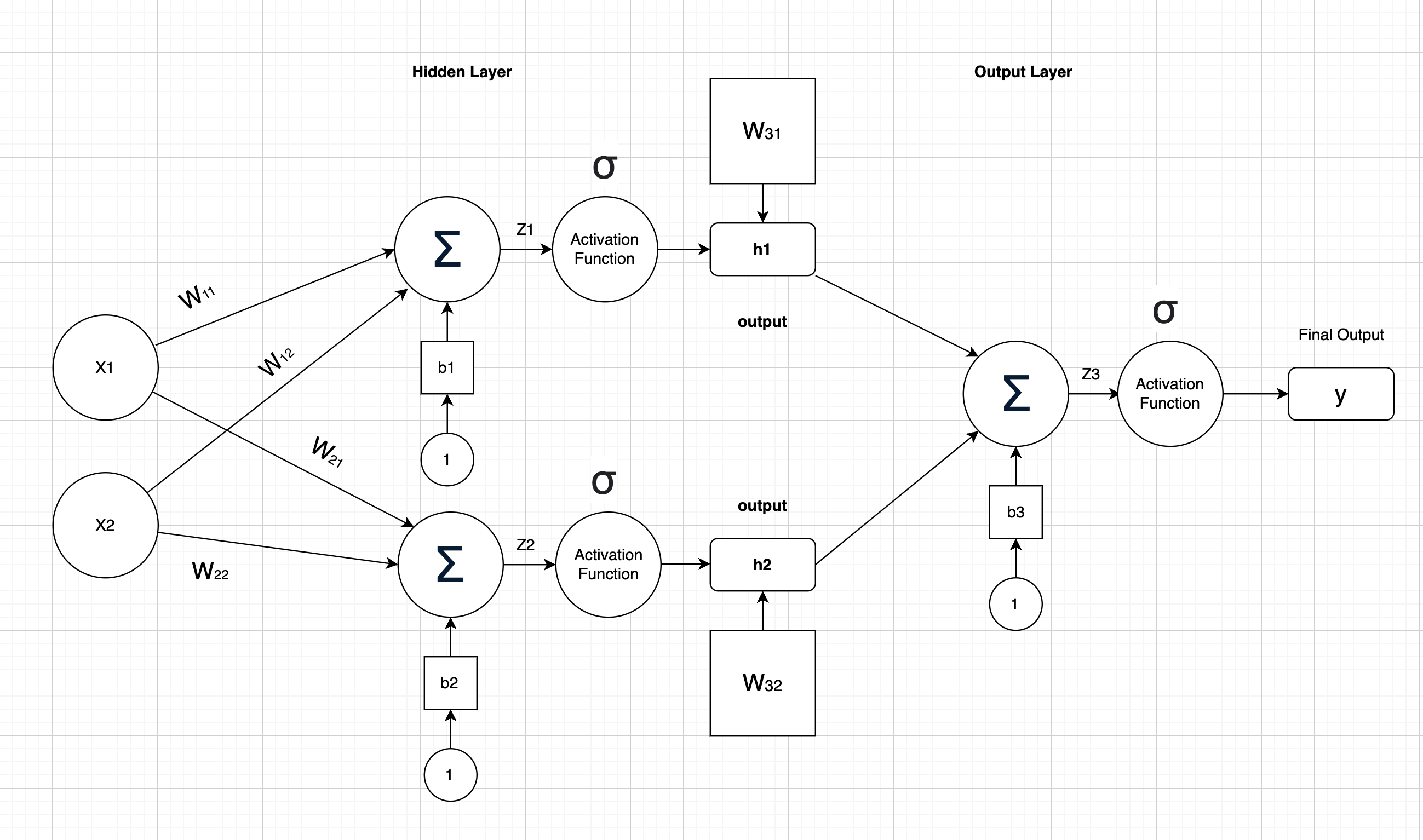
Let's consider a simple neural network with two inputs (\( x_1, x_2 \)), one hidden layer with two neurons, and one output neuron. We'll use the sigmoid activation function and mean squared error loss.

Forward Pass:

1. Compute hidden layer inputs:

\[ z_1 = w_{11}x_1 + w_{12}x_2 + b_1 \] \[ z_2 = w_{21}x_1 + w_{22}x_2 + b_2 \]

2. Apply activation to get hidden layer outputs:

\[ h_1 = \sigma(z_1), \quad h_2 = \sigma(z_2) \]

3. Compute output layer input:

\[ z_3 = w_{31}h_1 + w_{32}h_2 + b_3 \]

4. Apply activation to get network output:

\[ y = \sigma(z_3) \]

5. Calculate mean squared error loss:

\[ L = \frac{1}{2}(y - t)^2 \] \[\text{ Where t is the target output}\] \[\text{ and } \sigma \text { is the activation function (sigmoid in this case)}\]

Backward Pass:

1. Output layer error gradients:

\[ \frac{\partial L}{\partial y} = (y - t) \] \[ \frac{\partial y}{\partial z_3} = y(1-y) \]

2. Output layer weight and bias gradients:

\[ \frac{\partial L}{\partial w_{31}} = \frac{\partial L}{\partial y} \cdot \frac{\partial y}{\partial z_3} \cdot h_1 \] \[ \frac{\partial L}{\partial w_{32}} = \frac{\partial L}{\partial y} \cdot \frac{\partial y}{\partial z_3} \cdot h_2 \] \[ \frac{\partial L}{\partial b_3} = \frac{\partial L}{\partial y} \cdot \frac{\partial y}{\partial z_3} \]

3. Hidden layer error gradients (including activation derivatives):

\[ \frac{\partial L}{\partial h_1} = \frac{\partial L}{\partial y} \cdot \frac{\partial y}{\partial z_3} \cdot w_{31} \cdot h_1(1-h_1) \] \[ \frac{\partial L}{\partial h_2} = \frac{\partial L}{\partial y} \cdot \frac{\partial y}{\partial z_3} \cdot w_{32} \cdot h_2(1-h_2) \]

4. Hidden layer weight and bias gradients:

\[ \frac{\partial L}{\partial w_{11}} = \frac{\partial L}{\partial h_1} \cdot x_1, \quad \frac{\partial L}{\partial w_{12}} = \frac{\partial L}{\partial h_1} \cdot x_2, \quad \frac{\partial L}{\partial b_1} = \frac{\partial L}{\partial h_1} \] \[ \frac{\partial L}{\partial w_{21}} = \frac{\partial L}{\partial h_2} \cdot x_1, \quad \frac{\partial L}{\partial w_{22}} = \frac{\partial L}{\partial h_2} \cdot x_2, \quad \frac{\partial L}{\partial b_2} = \frac{\partial L}{\partial h_2} \]

The Training Process

After calculating gradients, we update each weight using the learning rate (\( \eta \)):

\( w_{\text{new}} = w_{\text{old}} - \eta \cdot \frac{\partial L}{\partial w} \)

This process is repeated for each training example, gradually minimizing the loss function and improving the network's predictions.

Weight Update Effects:

Each weight update creates a cascade of changes through the network. When we update a weight, the neuron's response changes, affecting all connected neurons in subsequent layers. This ripples through to the final output and transforms the overall loss landscape. For example, if we adjust \(w_{11}\) in our hidden layer: The activation \(h_1\) changes for the same input. This new \(h_1\) affects the weighted sum going into the output neuron and the output prediction shifts which then creates a new error gradient for the next training example.

However, in training neural networks, 1 example is not enough, it's about finding weights that work well across many examples. Here's what actually happens:

Batch Processing:

We process multiple examples in batches to find weights that perform well across the entire dataset. The batch gradient is:

\( \frac{\partial L_{\text{batch}}}{\partial w} = \frac{1}{n}\sum_{i=1}^n \frac{\partial L_i}{\partial w} \)

Training Progression:

In practice, we see that, early epochs see large weight adjustments and significant loss reduction as the network learns broad patterns. Middle epochs show more subtle refinements, while later epochs focus on fine-tuning. Training continues until:

The loss stabilizes across both training and validation sets
Weight updates become naturally smaller
The network shows good generalization performance