Neural Network

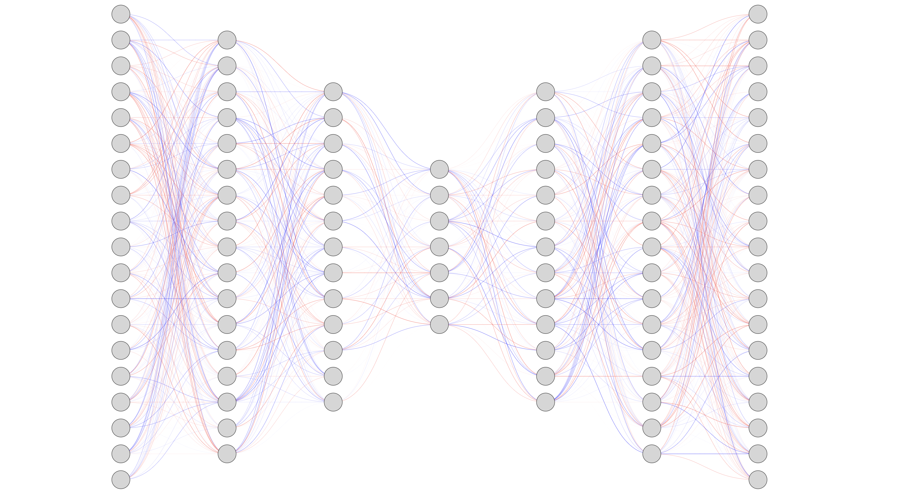
Neuron Model and Network Architectures

Single Neuron Perceptron

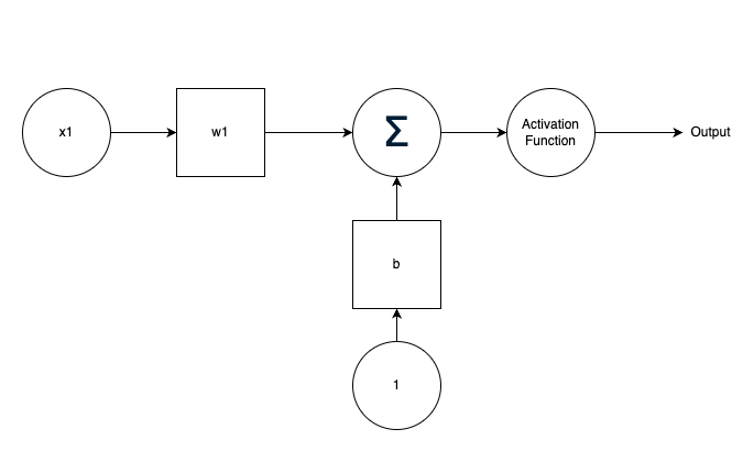
Here a scalar input x1 is multiplied by a scalar weight w1 to form w1*x1 which is fed to the summation function. A second input of 1 is multiplied by a bias term 'b' and then passed to the summation function. The summation function thus adds the two products together: w1*x1 + b*1. The output of this summation function is called a 'net input'. This 'net input' then goes into an Activation Function or a transfer function 'f' which produces a scalar neuron output.

If we want to relate this with biology, the idea here is that the weight w1 in this example relates to the strength of a synapse. The summation function and the transfer function represent the cell body of a neuron, and the neuron output represents the signal on the axon.

The neuron ouput is calculated as: output = f(w1*x1 + b)

Both w1 and b are adjustable scalar parameters of the neuron and will be adjusted by some learning rule so that the neuron model can produce a specific output.

Single Neuron Perceptron with 'n' inputs

The following diagram shows a neuron with multiple inputs.

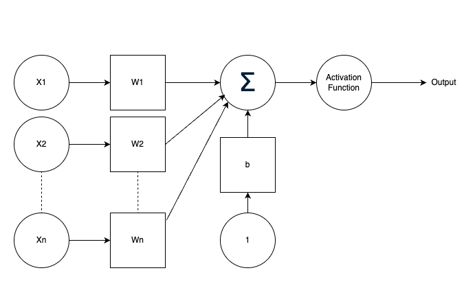
Its output is calculated similarly as above

net_input = w1*x1 + w2*x2 + ... + wn*xn + b

This expression can be written in a matrix form as:

net_input = WX + b

Where W is a matrix representation of the weights w1, w2, ... wn

\[ W = \begin{bmatrix} w_1 & w_2 & \dots & w_n \end{bmatrix} \]

and X is a vector representation of the inputs x1, x2, ... xn

\[ X = \begin{bmatrix} x_1 \\ x_2 \\ \vdots \\ x_n \end{bmatrix} \]

The resulting computation \( W X + b \) is:

\[\begin{bmatrix} w_1 & w_2 & \dots & w_n \end{bmatrix} \begin{bmatrix} x_1 \\x_2 \\\vdots \\x_n \end{bmatrix} + b \]

neuron output = f(WX + b)

A layer of Neurons with multiple inputs

Now let us take a look at a layer of neurons with multiple inputs:

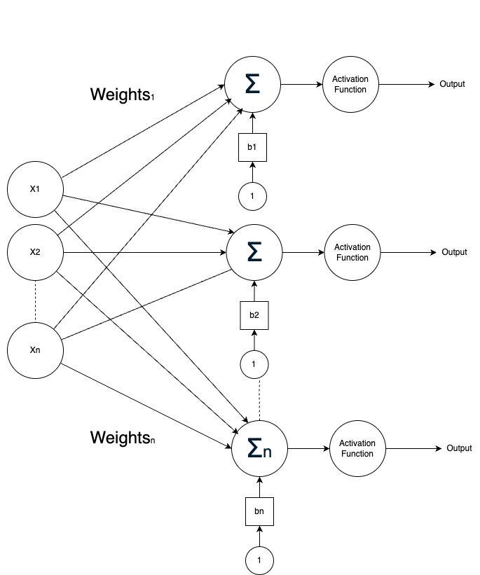
In this case, each neuron in the layer has its own set of weights and biases, but the operation for the entire layer can still be expressed in matrix form.

The computation for this layer can be written in matrix form as:

net_input = WX + b

Where:

\[ W = \begin{bmatrix} w_{11} & w_{12} & \dots & w_{1n} \\ w_{21} & w_{22} & \dots & w_{2n} \\ \vdots & \vdots & \ddots & \vdots \\ w_{m1} & w_{m2} & \dots & w_{mn} \end{bmatrix} \]

is the weights matrix for the layer, where \( m \) is the number of neurons in the layer, and \( n \) is the number of inputs.

\[ X = \begin{bmatrix} x_1 \\ x_2 \\ \vdots \\ x_n \end{bmatrix} \]

is the input vector, and:

\[ b = \begin{bmatrix} b_1 \\ b_2 \\ \vdots \\ b_m \end{bmatrix} \]

is the bias vector for the layer, where each \( b_i \) corresponds to a single neuron in the layer.

The resulting computation for the layer is:

\[ WX + b = \begin{bmatrix} w_{11} & w_{12} & \dots & w_{1n} \\ w_{21} & w_{22} & \dots & w_{2n} \\ \vdots & \vdots & \ddots & \vdots \\ w_{m1} & w_{m2} & \dots & w_{mn} \end{bmatrix} \begin{bmatrix} x_1 \\ x_2 \\ \vdots \\ x_n \end{bmatrix} + \begin{bmatrix} b_1 \\ b_2 \\ \vdots \\ b_m \end{bmatrix} \]

Finally, the output of the layer is calculated by applying an activation function \( f \) to each element of \( WX + b \):

\[ \text{layer output} = f(WX + b) \]

Multi Layer Neural Network

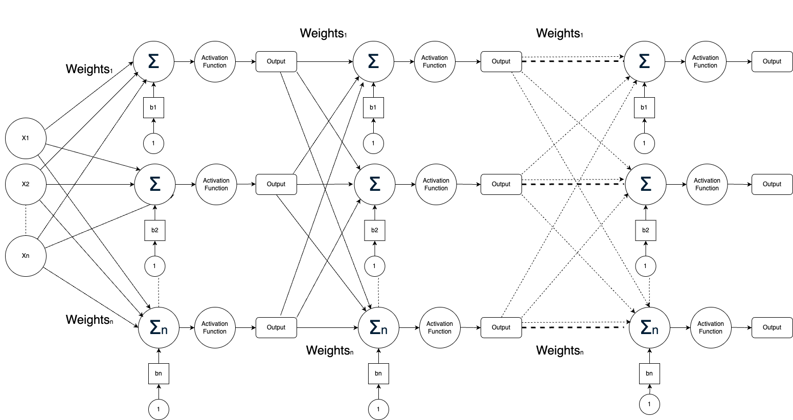
A multi-layer neural network consists of multiple layers of neurons, where the output of one layer serves as the input to the next layer. The computation for each layer can be represented in matrix form, enabling efficient calculations across the network.

For a neural network with \( L \) layers, let:

• \( W^{[l]} \): the weights matrix for layer \( l \), where \( l = 1, 2, \dots, L \).
• \( b^{[l]} \): the bias vector for layer \( l \).
• \( X^{[l-1]} \): the input to layer \( l \) (output of the previous layer, with \( X^{[0]} \) being the input vector to the network).
• \( Z^{[l]} \): the weighted sum before applying the activation function in layer \( l \).
• \( X^{[l]} \): the output of layer \( l \) after applying the activation function \( f^{[l]} \).

The computation for layer \( l \) is as follows:

\[ Z^{[l]} = W^{[l]} X^{[l-1]} + b^{[l]} \]

Where:

\[ W^{[l]} = \begin{bmatrix} w^{[l]}_{11} & w^{[l]}_{12} & \dots & w^{[l]}_{1n} \\ w^{[l]}_{21} & w^{[l]}_{22} & \dots & w^{[l]}_{2n} \\ \vdots & \vdots & \ddots & \vdots \\ w^{[l]}_{m1} & w^{[l]}_{m2} & \dots & w^{[l]}_{mn} \end{bmatrix} \]

is the weights matrix for layer \( l \) (size: \( m \times n \), where \( m \) is the number of neurons in the current layer and \( n \) is the number of inputs to that layer).

\[ b^{[l]} = \begin{bmatrix} b^{[l]}_1 \\ b^{[l]}_2 \\ \vdots \\ b^{[l]}_m \end{bmatrix} \]

is the bias vector for layer \( l \) (size: \( m \times 1 \)).

\[ X^{[l-1]} = \begin{bmatrix} x^{[l-1]}_1 \\ x^{[l-1]}_2 \\ \vdots \\ x^{[l-1]}_n \end{bmatrix} \]

is the input vector to layer \( l \) (size: \( n \times 1 \)).

After calculating \( Z^{[l]} \), the activation function \( f^{[l]} \) is applied element-wise to compute the output of layer \( l \):

\[ X^{[l]} = f^{[l]}(Z^{[l]}) \]

The output of the final layer \( X^{[L]} \) is the output of the neural network.

Incorporating Bias into the Weight Matrix

In practice, it is often easy to incorporate the bias term \( b \) into the weight matrix \( W \) by including an additional input to the network with a fixed value of 1, called the bias input. What this allows us to do is to do the computation in a matrix form without explicitly handling the bias separately.

To do this, we modify the weights and inputs as follows:

Modified Weight Matrix: we simply add an extra column at the beginning of \( W \), corresponding to the bias weights:

\[ W_{\text{augmented}} = \begin{bmatrix} b_1 & w_{11} & w_{12} & \dots & w_{1n} \\ b_2 & w_{21} & w_{22} & \dots & w_{2n} \\ \vdots & \vdots & \vdots & \ddots & \vdots \\ b_m & w_{m1} & w_{m2} & \dots & w_{mn} \end{bmatrix} \]

Modified Input Vector: Add a constant input of 1 as the first entry in \( X \):

\[ X_{\text{augmented}} = \begin{bmatrix} 1 \\ x_1 \\ x_2 \\ \vdots \\ x_n \end{bmatrix} \]

and then the computation simply reduces to:

\[ \quad W_{\text{augmented}} * X_{\text{augmented}}\]

\[ \quad \begin{bmatrix} b_1 & w_{11} & w_{12} & \dots & w_{1n} \\ b_2 & w_{21} & w_{22} & \dots & w_{2n} \\ \vdots & \vdots & \vdots & \ddots & \vdots \\ b_m & w_{m1} & w_{m2} & \dots & w_{mn} \end{bmatrix} * \begin{bmatrix} 1 \\ x_1 \\ x_2 \\ \vdots \\ x_n \end{bmatrix} \]